XArray: the power of pandas for multidimensional arrays

http://xarray.pydata.org

Robin Wilson

@sciremotesense       robin@rtwilson.com

Slides: http://bit.do/xarray_pyconuk

Code: https://github.com/robintw/XArray_PyConUK2018

Satellite air quality data (from the MODIS MAIAC product)

Problem

We have many decades of daily raster data, and want to get:

• Seasonal means and standard deviations

• Long time-series across specific points

• Individual images at specific times

The 'simple' solution

• Load in the image data (using GDAL or rasterio)

• Store in a large 3D numpy array (dimensions: X, Y and time)

• Index, slice and dice the array...

Not as easy it sounds...need to keep track of everything!

Enter XArray

The power of pandas for multidimensional arrays

import xarray as xr

Quick example

PM25 = xr.open_dataarray('/Users/robin/code/MAIACProcessing/All2014.nc')

PM25.shape

(181, 1162, 1240)

PM25.dims

('time', 'y', 'x')

seasonal = PM25.groupby('time.season').mean(dim='time')

seasonal.plot.imshow(col='season', robust=True)

<xarray.plot.facetgrid.FacetGrid at 0x30d4aceb8>

time_series = PM25.isel(x=1000, y=1100).to_pandas().dropna()

time_series

time
2014-01-07     62.0
2014-01-17    121.0
2014-01-25    127.0
2014-02-10    135.0
2014-02-11    186.0
2014-02-18    237.0
2014-02-25    352.0
2014-02-26    293.0
2014-02-27    260.0
2014-03-01    165.0
2014-03-08    221.0
2014-03-09    221.0
2014-03-10    291.0
2014-03-13    552.0
2014-03-16    156.0
2014-03-21    159.0
2014-03-22    160.0
2014-03-23    163.0
2014-03-25    261.0
2014-03-30    362.0
2014-04-04     19.0
2014-04-09     19.0
2014-04-10     19.0
2014-04-11     19.0
2014-04-13     33.0
2014-04-14     19.0
2014-04-16    159.0
2014-04-18     53.0
2014-04-19    118.0
2014-04-24    194.0
2014-04-25    250.0
2014-05-10    154.0
2014-05-13    181.0
2014-05-14     19.0
2014-05-15    117.0
2014-05-17    239.0
2014-05-22    188.0
2014-06-02    189.0
2014-06-05     71.0
2014-06-07    107.0
2014-06-13    115.0
2014-06-14    324.0
2014-06-15     64.0
2014-06-18    132.0
2014-06-20    101.0
2014-06-21    115.0
2014-06-23    200.0
2014-06-27    162.0
dtype: float32

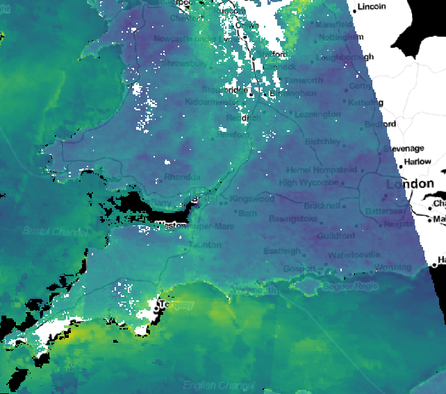
one_day = PM25.sel(time='2014-02-15')

one_day.plot(robust=True)

<matplotlib.collections.QuadMesh at 0x31dcdeba8>

Summary

seasonal = PM25.groupby('time.season').mean(dim='time')

time_series = PM25.isel(x=1000, y=1100).to_pandas().dropna()

one_day = PM25.sel(time='2014-02-20')

Introduction to XArray

xarray.DataArray is a fancy, labelled version of a numpy.ndarray

xarray.Dataset is a collection of multiple DataArrays which share dimensions

(A Dataset is a representation of a NetCDF file)

arr = np.random.rand(3, 4, 2)

xr.DataArray(arr)

<xarray.DataArray (dim_0: 3, dim_1: 4, dim_2: 2)>
array([[[0.006194, 0.380531],
        [0.561032, 0.360739],
        [0.515117, 0.300988],
        [0.650297, 0.560798]],

       [[0.703038, 0.762046],
        [0.703794, 0.467468],
        [0.19292 , 0.395919],
        [0.344915, 0.874793]],

       [[0.570962, 0.881131],
        [0.758426, 0.582632],
        [0.419739, 0.634596],
        [0.720827, 0.12582 ]]])
Dimensions without coordinates: dim_0, dim_1, dim_2

xr.DataArray(arr, dims=('x', 'y', 'time'))

<xarray.DataArray (x: 3, y: 4, time: 2)>
array([[[0.006194, 0.380531],
        [0.561032, 0.360739],
        [0.515117, 0.300988],
        [0.650297, 0.560798]],

       [[0.703038, 0.762046],
        [0.703794, 0.467468],
        [0.19292 , 0.395919],
        [0.344915, 0.874793]],

       [[0.570962, 0.881131],
        [0.758426, 0.582632],
        [0.419739, 0.634596],
        [0.720827, 0.12582 ]]])
Dimensions without coordinates: x, y, time

da = xr.DataArray(arr,
                  dims=('x', 'y', 'time'),
                  coords={'x': [10, 20, 30],
                          'y': [0.3, 0.7, 1.3, 1.5],
                          'time': [datetime.datetime(2016, 3, 5),
                                   datetime.datetime(2016, 4, 7)]})

da

<xarray.DataArray (x: 3, y: 4, time: 2)>
array([[[0.006194, 0.380531],
        [0.561032, 0.360739],
        [0.515117, 0.300988],
        [0.650297, 0.560798]],

       [[0.703038, 0.762046],
        [0.703794, 0.467468],
        [0.19292 , 0.395919],
        [0.344915, 0.874793]],

       [[0.570962, 0.881131],
        [0.758426, 0.582632],
        [0.419739, 0.634596],
        [0.720827, 0.12582 ]]])
Coordinates:
  * x        (x) int64 10 20 30
  * y        (y) float64 0.3 0.7 1.3 1.5
  * time     (time) datetime64[ns] 2016-03-05 2016-04-07

da.sel(time='2016-03-05')

<xarray.DataArray (x: 3, y: 4)>
array([[0.006194, 0.561032, 0.515117, 0.650297],
       [0.703038, 0.703794, 0.19292 , 0.344915],
       [0.570962, 0.758426, 0.419739, 0.720827]])
Coordinates:
  * x        (x) int64 10 20 30
  * y        (y) float64 0.3 0.7 1.3 1.5
    time     datetime64[ns] 2016-03-05

da.isel(time=1)

<xarray.DataArray (x: 3, y: 4)>
array([[0.380531, 0.360739, 0.300988, 0.560798],
       [0.762046, 0.467468, 0.395919, 0.874793],
       [0.881131, 0.582632, 0.634596, 0.12582 ]])
Coordinates:
  * x        (x) int64 10 20 30
  * y        (y) float64 0.3 0.7 1.3 1.5
    time     datetime64[ns] 2016-04-07

da.sel(x=slice(0, 20))

<xarray.DataArray (x: 2, y: 4, time: 2)>
array([[[0.006194, 0.380531],
        [0.561032, 0.360739],
        [0.515117, 0.300988],
        [0.650297, 0.560798]],

       [[0.703038, 0.762046],
        [0.703794, 0.467468],
        [0.19292 , 0.395919],
        [0.344915, 0.874793]]])
Coordinates:
  * x        (x) int64 10 20
  * y        (y) float64 0.3 0.7 1.3 1.5
  * time     (time) datetime64[ns] 2016-03-05 2016-04-07

da.mean(dim='time')

<xarray.DataArray (x: 3, y: 4)>
array([[0.193362, 0.460886, 0.408053, 0.605548],
       [0.732542, 0.585631, 0.294419, 0.609854],
       [0.726047, 0.670529, 0.527168, 0.423323]])
Coordinates:
  * x        (x) int64 10 20 30
  * y        (y) float64 0.3 0.7 1.3 1.5

da.mean(dim=['x', 'y'])

<xarray.DataArray (time: 2)>
array([0.512272, 0.527288])
Coordinates:
  * time     (time) datetime64[ns] 2016-03-05 2016-04-07

PM25.sel(time='2014').groupby('time.month').std(dim='time')

<xarray.DataArray 'data' (month: 6, y: 1162, x: 1240)>
array([[[      nan,       nan, ...,       nan,       nan],
        [      nan,       nan, ...,       nan,       nan],
        ...,
        [      nan,       nan, ...,       nan,       nan],
        [      nan,       nan, ...,       nan,       nan]],

       [[      nan,       nan, ...,       nan,       nan],
        [  0.     ,       nan, ...,       nan,       nan],
        ...,
        [      nan,       nan, ...,       nan,       nan],
        [      nan,       nan, ...,       nan,       nan]],

       ...,

       [[ 23.97684,   0.     , ...,       nan,       nan],
        [  1.     ,   2.5    , ...,       nan,       nan],
        ...,
        [      nan,       nan, ...,       nan,       nan],
        [      nan,       nan, ...,       nan,       nan]],

       [[146.48776, 125.04899, ...,       nan,       nan],
        [146.27904, 148.14934, ...,       nan,       nan],
        ...,
        [      nan,       nan, ...,       nan,       nan],
        [      nan,       nan, ...,       nan,       nan]]], dtype=float32)
Coordinates:
  * y        (y) float64 1.429e+06 1.428e+06 1.427e+06 1.426e+06 1.424e+06 ...
  * x        (x) float64 -9.476e+05 -9.464e+05 -9.451e+05 -9.439e+05 ...
  * month    (month) int64 1 2 3 4 5 6

Efficient processing with dask and dask.distributed

dask creates a computational graph of your processing steps, and then executes it as efficiently as possible.

This includes only loading data that is actually needed and only processing things once.

data = xr.open_mfdataset(['DaskTest1.nc', 'DaskTest2.nc'], chunks={'time':10})['data']
avg = data.mean(dim='time')

Dask execution graph

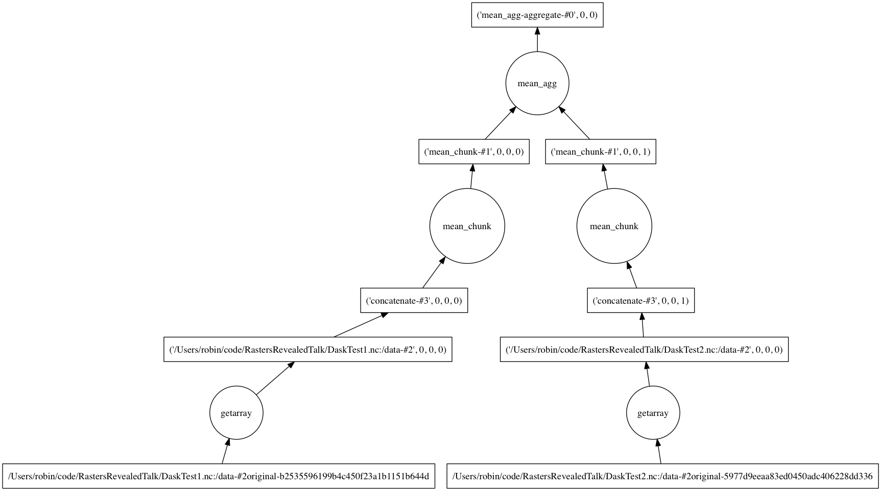
seasonal = data.groupby('time.season').mean(dim='time')

Dask execution graph

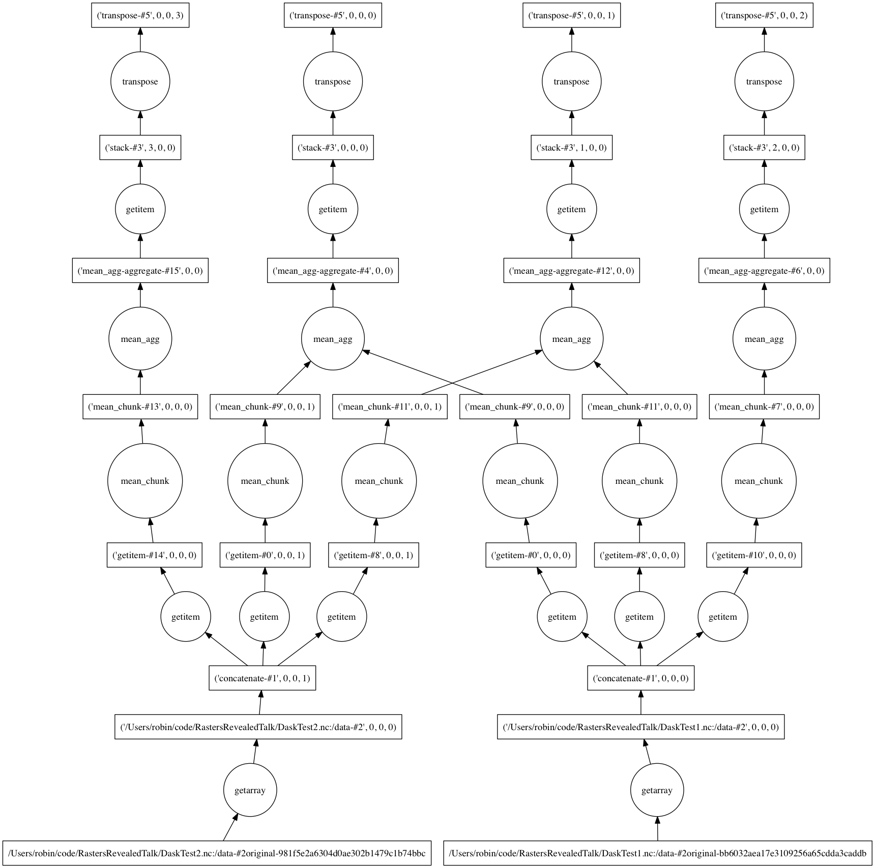
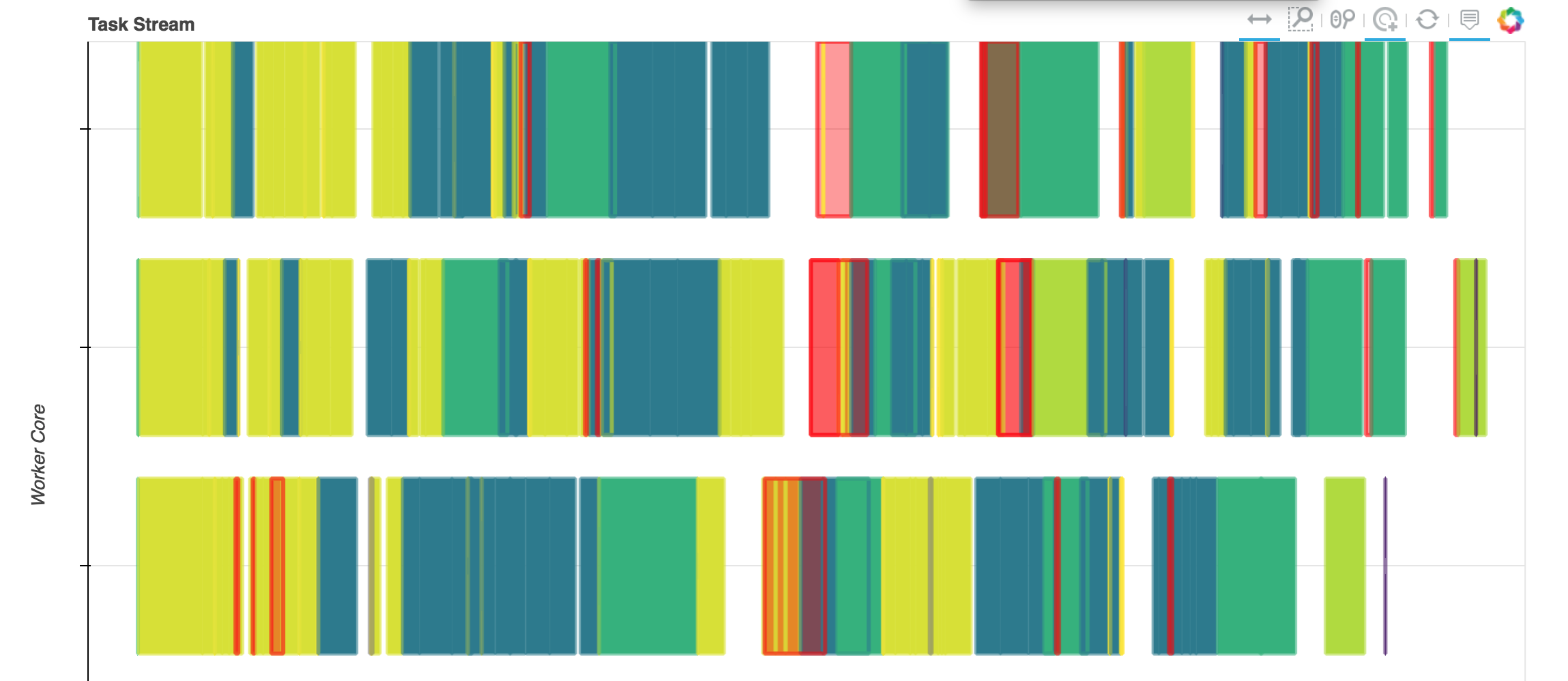
dask.distributed

All of these different chunks, and separate processing chains can be run on separate processes or separate computers.

Getting data into xarray

xarray can read various formats directly:

• NetCDF
• HDF
• GRIB

xarray can now use rasterio to read loads of geographic raster formats

xr.open_rasterio('satellite_image.tif')

<xarray.DataArray (band: 3, y: 1644, x: 1435)>
[7077420 values with dtype=uint8]
Coordinates:
  * band     (band) int64 1 2 3
  * y        (y) float64 1.484e+05 1.484e+05 1.484e+05 1.484e+05 1.484e+05 ...
  * x        (x) float64 4.301e+05 4.301e+05 4.302e+05 4.302e+05 4.302e+05 ...
Attributes:
    transform:   (10.0, 0.0, 430130.2396, 0.0, -10.0, 148415.8755, 0.0, 0.0, ...
    crs:         +ellps=airy +k=0.999601 +lat_0=49 +lon_0=-2 +no_defs +proj=t...
    res:         (10.0, 10.0)
    is_tiled:    0
    nodatavals:  (nan, nan, nan)

Example - combining multiple satellite data files into a time-series

Take a large number of files, one from each orbit of a satellite, and put them into one large array with a time dimension.

def file_to_da(filename):
    da = xr.open_rasterio(filename)
    
    time_str = os.path.basename(filename)[17:-17]
    time_obj = datetime.datetime.strptime(time_str, '%Y%j%H%M')
    da.coords['time'] = time_obj
    
    return da.isel(band=0)

list_of_data_arrays = [file_to_da(filename) for filename in files]

combined = xr.concat(list_of_data_arrays, dim='time')

combined.shape

(10, 1162, 1240)

combined.coords

Coordinates:
    band     int64 1
  * y        (y) float64 1.429e+06 1.427e+06 1.426e+06 1.425e+06 1.424e+06 ...
  * x        (x) float64 -9.47e+05 -9.458e+05 -9.445e+05 -9.432e+05 ...
  * time     (time) datetime64[ns] 2003-04-16T14:40:00 2002-03-19T11:20:00 ...

Getting raster data out of xarray

from xarray_to_rasterio import xarray_to_rasterio

mean = combined.mean(dim='time', keep_attrs=True)

xarray_to_rasterio(mean, 'Mean.tif')

A few tasters...

Interpolation

PM25.interp(x=318193.5, y=176849.7).to_pandas().dropna().head()

time
2014-01-07    74.390257
2014-01-09    42.588762
2014-01-19    84.464250
2014-02-07    37.803606
2014-02-11    67.395553
dtype: float64

PM25.interp(x=318193.5, y=176849.7, method='nearest').to_pandas().dropna().head()

time
2014-01-07     72.0
2014-01-09     42.0
2014-01-19     82.0
2014-01-27    159.0
2014-02-01    297.0
dtype: float32

Resampling time series

PM25.resample(time='1M').mean(dim='time')

<xarray.DataArray 'data' (time: 6, y: 1162, x: 1240)>
array([[[       nan,        nan, ...,        nan,        nan],
        [       nan,        nan, ...,        nan,        nan],
        ...,
        [       nan,        nan, ...,        nan,        nan],
        [       nan,        nan, ...,        nan,        nan]],

       [[       nan,        nan, ...,        nan,        nan],
        [ 20.      ,        nan, ...,        nan,        nan],
        ...,
        [       nan,        nan, ...,        nan,        nan],
        [       nan,        nan, ...,        nan,        nan]],

       ...,

       [[ 70.333336,  46.      , ...,        nan,        nan],
        [ 49.      ,  53.5     , ...,        nan,        nan],
        ...,
        [       nan,        nan, ...,        nan,        nan],
        [       nan,        nan, ...,        nan,        nan]],

       [[333.      , 326.5     , ...,        nan,        nan],
        [324.33334 , 334.33334 , ...,        nan,        nan],
        ...,
        [       nan,        nan, ...,        nan,        nan],
        [       nan,        nan, ...,        nan,        nan]]], dtype=float32)
Coordinates:
  * time     (time) datetime64[ns] 2014-01-31 2014-02-28 2014-03-31 ...
  * y        (y) float64 1.429e+06 1.428e+06 1.427e+06 1.426e+06 1.424e+06 ...
  * x        (x) float64 -9.476e+05 -9.464e+05 -9.451e+05 -9.439e+05 ...

Rolling windows

PM25.rolling(time=5).mean()

<xarray.DataArray (time: 10, y: 1162, x: 1240)>
array([[[nan, nan, ..., nan, nan],
        [nan, nan, ..., nan, nan],
        ...,
        [nan, nan, ..., nan, nan],
        [nan, nan, ..., nan, nan]],

       [[nan, nan, ..., nan, nan],
        [nan, nan, ..., nan, nan],
        ...,
        [nan, nan, ..., nan, nan],
        [nan, nan, ..., nan, nan]],

       ...,

       [[nan, nan, ..., nan, nan],
        [nan, nan, ..., nan, nan],
        ...,
        [nan, nan, ..., nan, nan],
        [nan, nan, ..., nan, nan]],

       [[nan, nan, ..., nan, nan],
        [nan, nan, ..., nan, nan],
        ...,
        [nan, nan, ..., nan, nan],
        [nan, nan, ..., nan, nan]]], dtype=float32)
Coordinates:
    band     int64 1
  * y        (y) float64 1.429e+06 1.427e+06 1.426e+06 1.425e+06 1.424e+06 ...
  * x        (x) float64 -9.47e+05 -9.458e+05 -9.445e+05 -9.432e+05 ...
  * time     (time) datetime64[ns] 2003-04-16T14:40:00 2002-03-19T11:20:00 ...

OPeNDAP

Accessing data over the internet - but only downloading the bits you use

dataset = xr.open_dataset('http://opendap.knmi.nl/knmi/thredds/dodsC/e-obs_0.25regular/tg_0.25deg_reg_v17.0.nc')

dataset['tg']

<xarray.DataArray 'tg' (time: 24837, latitude: 201, longitude: 464)>
[2316397968 values with dtype=float32]
Coordinates:
  * longitude  (longitude) float32 -40.375 -40.125 -39.875 -39.625 -39.375 ...
  * latitude   (latitude) float32 25.375 25.625 25.875 26.125 26.375 26.625 ...
  * time       (time) datetime64[ns] 1950-01-01 1950-01-02 1950-01-03 ...
Attributes:
    long_name:      mean temperature
    units:          Celsius
    standard_name:  air_temperature

temperature = dataset['tg']
oneday = temperature.sel(time='2009-07-01')
oneday.plot(robust=True)

<matplotlib.collections.QuadMesh at 0x324b65080>

xarray extensions

• Simulation models in xarray (xarray-simlab)

• WRF Weather Forecasting Model functions (wrf-python)

• Empirical Orthogonal Functions (eofs)

• Many more at http://xarray.pydata.org/en/stable/faq.html#what-other-projects-leverage-xarray

from eofs.xarray import Eof
monthly = PM25.resample(time='M').mean('time')
solver = Eof(monthly)
results = solver.eofs()

results.plot(col='mode', col_wrap=3, robust=True)

<xarray.plot.facetgrid.FacetGrid at 0x324a77550>

Resources

Slides: http://bit.do/xarray_pyconuk

Code: https://github.com/robintw/XArray_PyConUK2018

XArray docs: http://xarray.pydata.org/

robin@rtwilson.com       @sciremotesense       @robintw on Slack