Raster processing with XArray

Robin Wilson

Geography & Environment, University of Southampton

@sciremotesense       robin@rtwilson.com

Problem

Processing large time series of raster data is difficult

Example:

We have many decades of daily raster data, and want to get:

  • Seasonal means and standard deviations
  • Long time-series across specific points
  • Individual images at specific times

XArray

The power of pandas for multidimensional arrays

  • Labelled
  • Multidimensional
  • Efficient
  • Easy to use!
  • python (obviously!)
  • numpy
  • pandas
  • matplotlib
  • GDAL
  • rasterio

Previous experience?

Q: How many people are experienced with numpy?

Q: ...with pandas?

Q: ...with GDAL?

In [2]:
import xarray as xr

Example

In [3]:
PM25 = xr.open_dataarray('/Users/robin/code/MAIACProcessing/All2014.nc')
In [4]:
PM25.shape
Out[4]:
(181, 1162, 1240)
In [5]:
PM25.dims
Out[5]:
(u'time', u'y', u'x')
In [6]:
seasonal = PM25.groupby('time.season').mean(dim='time')
In [7]:
seasonal.plot.imshow(col='season', robust=True)
Out[7]:
<xarray.plot.facetgrid.FacetGrid at 0x10cddea10>
In [8]:
time_series = PM25.isel(x=1000, y=1100).to_pandas().dropna()
In [9]:
time_series
Out[9]:
time
2014-01-07     62.0
2014-01-17    121.0
2014-01-25    127.0
2014-02-10    135.0
2014-02-11    186.0
2014-02-18    237.0
2014-02-25    352.0
2014-02-26    293.0
2014-02-27    260.0
2014-03-01    165.0
2014-03-08    221.0
2014-03-09    221.0
2014-03-10    291.0
2014-03-13    552.0
2014-03-16    156.0
2014-03-21    159.0
2014-03-22    160.0
2014-03-23    163.0
2014-03-25    261.0
2014-03-30    362.0
2014-04-04     19.0
2014-04-09     19.0
2014-04-10     19.0
2014-04-11     19.0
2014-04-13     33.0
2014-04-14     19.0
2014-04-16    159.0
2014-04-18     53.0
2014-04-19    118.0
2014-04-24    194.0
2014-04-25    250.0
2014-05-10    154.0
2014-05-13    181.0
2014-05-14     19.0
2014-05-15    117.0
2014-05-17    239.0
2014-05-22    188.0
2014-06-02    189.0
2014-06-05     71.0
2014-06-07    107.0
2014-06-13    115.0
2014-06-14    324.0
2014-06-15     64.0
2014-06-18    132.0
2014-06-20    101.0
2014-06-21    115.0
2014-06-23    200.0
2014-06-27    162.0
dtype: float32
In [10]:
one_day = PM25.sel(time='2014-02-20')
In [11]:
one_day.plot(robust=True)
Out[11]:
<matplotlib.collections.QuadMesh at 0x119e41c90>

Summary

In [12]:
seasonal = PM25.groupby('time.season').mean(dim='time')
In [13]:
time_series = PM25.isel(x=1000, y=1100).to_pandas().dropna()
In [14]:
one_day = PM25.sel(time='2014-02-20')

Plan

  • Introduction to XArray
  • Efficient processing with dask and dask.distributed
  • Getting raster data into and out of XArray
  • Geographic processing
  • Where next...?

Introduction to XArray

xarray.DataArray is a fancy, labelled version of a numpy.ndarray

xarray.Dataset is a collection of multiple DataArrays which share dimensions

In [15]:
arr = np.random.rand(3, 4, 2)
In [16]:
xr.DataArray(arr)
Out[16]:
<xarray.DataArray (dim_0: 3, dim_1: 4, dim_2: 2)>
array([[[ 0.530635,  0.049118],
        [ 0.709483,  0.162677],
        [ 0.838245,  0.956551],
        [ 0.724748,  0.834736]],

       [[ 0.743153,  0.307386],
        [ 0.823829,  0.570499],
        [ 0.629053,  0.018669],
        [ 0.896682,  0.702414]],

       [[ 0.167959,  0.295538],
        [ 0.394742,  0.947428],
        [ 0.700852,  0.312621],
        [ 0.276099,  0.253416]]])
Dimensions without coordinates: dim_0, dim_1, dim_2
In [17]:
xr.DataArray(arr, dims=('x', 'y', 'time'))
Out[17]:
<xarray.DataArray (x: 3, y: 4, time: 2)>
array([[[ 0.530635,  0.049118],
        [ 0.709483,  0.162677],
        [ 0.838245,  0.956551],
        [ 0.724748,  0.834736]],

       [[ 0.743153,  0.307386],
        [ 0.823829,  0.570499],
        [ 0.629053,  0.018669],
        [ 0.896682,  0.702414]],

       [[ 0.167959,  0.295538],
        [ 0.394742,  0.947428],
        [ 0.700852,  0.312621],
        [ 0.276099,  0.253416]]])
Dimensions without coordinates: x, y, time
In [18]:
da = xr.DataArray(arr,
                  dims=('x', 'y', 'time'),
                  coords={'x': [10, 20, 30],
                          'y': [0.3, 0.7, 1.3, 1.5],
                          'time': [datetime.datetime(2016, 3, 5),
                                   datetime.datetime(2016, 4, 7)]})
In [19]:
da
Out[19]:
<xarray.DataArray (x: 3, y: 4, time: 2)>
array([[[ 0.530635,  0.049118],
        [ 0.709483,  0.162677],
        [ 0.838245,  0.956551],
        [ 0.724748,  0.834736]],

       [[ 0.743153,  0.307386],
        [ 0.823829,  0.570499],
        [ 0.629053,  0.018669],
        [ 0.896682,  0.702414]],

       [[ 0.167959,  0.295538],
        [ 0.394742,  0.947428],
        [ 0.700852,  0.312621],
        [ 0.276099,  0.253416]]])
Coordinates:
  * y        (y) float64 0.3 0.7 1.3 1.5
  * x        (x) int64 10 20 30
  * time     (time) datetime64[ns] 2016-03-05 2016-04-07
In [20]:
da.sel(time='2016-03-05')
Out[20]:
<xarray.DataArray (x: 3, y: 4)>
array([[ 0.530635,  0.709483,  0.838245,  0.724748],
       [ 0.743153,  0.823829,  0.629053,  0.896682],
       [ 0.167959,  0.394742,  0.700852,  0.276099]])
Coordinates:
  * y        (y) float64 0.3 0.7 1.3 1.5
  * x        (x) int64 10 20 30
    time     datetime64[ns] 2016-03-05
In [21]:
da.isel(time=1)
Out[21]:
<xarray.DataArray (x: 3, y: 4)>
array([[ 0.049118,  0.162677,  0.956551,  0.834736],
       [ 0.307386,  0.570499,  0.018669,  0.702414],
       [ 0.295538,  0.947428,  0.312621,  0.253416]])
Coordinates:
  * y        (y) float64 0.3 0.7 1.3 1.5
  * x        (x) int64 10 20 30
    time     datetime64[ns] 2016-04-07
In [22]:
da.sel(x=slice(0, 20))
Out[22]:
<xarray.DataArray (x: 2, y: 4, time: 2)>
array([[[ 0.530635,  0.049118],
        [ 0.709483,  0.162677],
        [ 0.838245,  0.956551],
        [ 0.724748,  0.834736]],

       [[ 0.743153,  0.307386],
        [ 0.823829,  0.570499],
        [ 0.629053,  0.018669],
        [ 0.896682,  0.702414]]])
Coordinates:
  * y        (y) float64 0.3 0.7 1.3 1.5
  * x        (x) int64 10 20
  * time     (time) datetime64[ns] 2016-03-05 2016-04-07
In [23]:
da.mean(dim='time')
Out[23]:
<xarray.DataArray (x: 3, y: 4)>
array([[ 0.289876,  0.43608 ,  0.897398,  0.779742],
       [ 0.525269,  0.697164,  0.323861,  0.799548],
       [ 0.231749,  0.671085,  0.506736,  0.264758]])
Coordinates:
  * y        (y) float64 0.3 0.7 1.3 1.5
  * x        (x) int64 10 20 30
In [24]:
da.mean(dim=['x', 'y'])
Out[24]:
<xarray.DataArray (time: 2)>
array([ 0.619623,  0.450921])
Coordinates:
  * time     (time) datetime64[ns] 2016-03-05 2016-04-07
In [25]:
PM25.sel(time='2014').groupby('time.month').std(dim='time')
Out[25]:
<xarray.DataArray u'data' (month: 6, y: 1162, x: 1240)>
array([[[        nan,         nan, ...,         nan,         nan],
        [        nan,         nan, ...,         nan,         nan],
        ..., 
        [        nan,         nan, ...,         nan,         nan],
        [        nan,         nan, ...,         nan,         nan]],

       [[        nan,         nan, ...,         nan,         nan],
        [   0.      ,         nan, ...,         nan,         nan],
        ..., 
        [        nan,         nan, ...,         nan,         nan],
        [        nan,         nan, ...,         nan,         nan]],

       ..., 
       [[  23.976839,    0.      , ...,         nan,         nan],
        [   1.      ,    2.5     , ...,         nan,         nan],
        ..., 
        [        nan,         nan, ...,         nan,         nan],
        [        nan,         nan, ...,         nan,         nan]],

       [[ 146.487762,  125.048988, ...,         nan,         nan],
        [ 146.279037,  148.149338, ...,         nan,         nan],
        ..., 
        [        nan,         nan, ...,         nan,         nan],
        [        nan,         nan, ...,         nan,         nan]]], dtype=float32)
Coordinates:
  * y        (y) float64 1.429e+06 1.428e+06 1.427e+06 1.426e+06 1.424e+06 ...
  * x        (x) float64 -9.476e+05 -9.464e+05 -9.451e+05 -9.439e+05 ...
  * month    (month) int64 1 2 3 4 5 6

Efficient processing with dask and dask.distributed

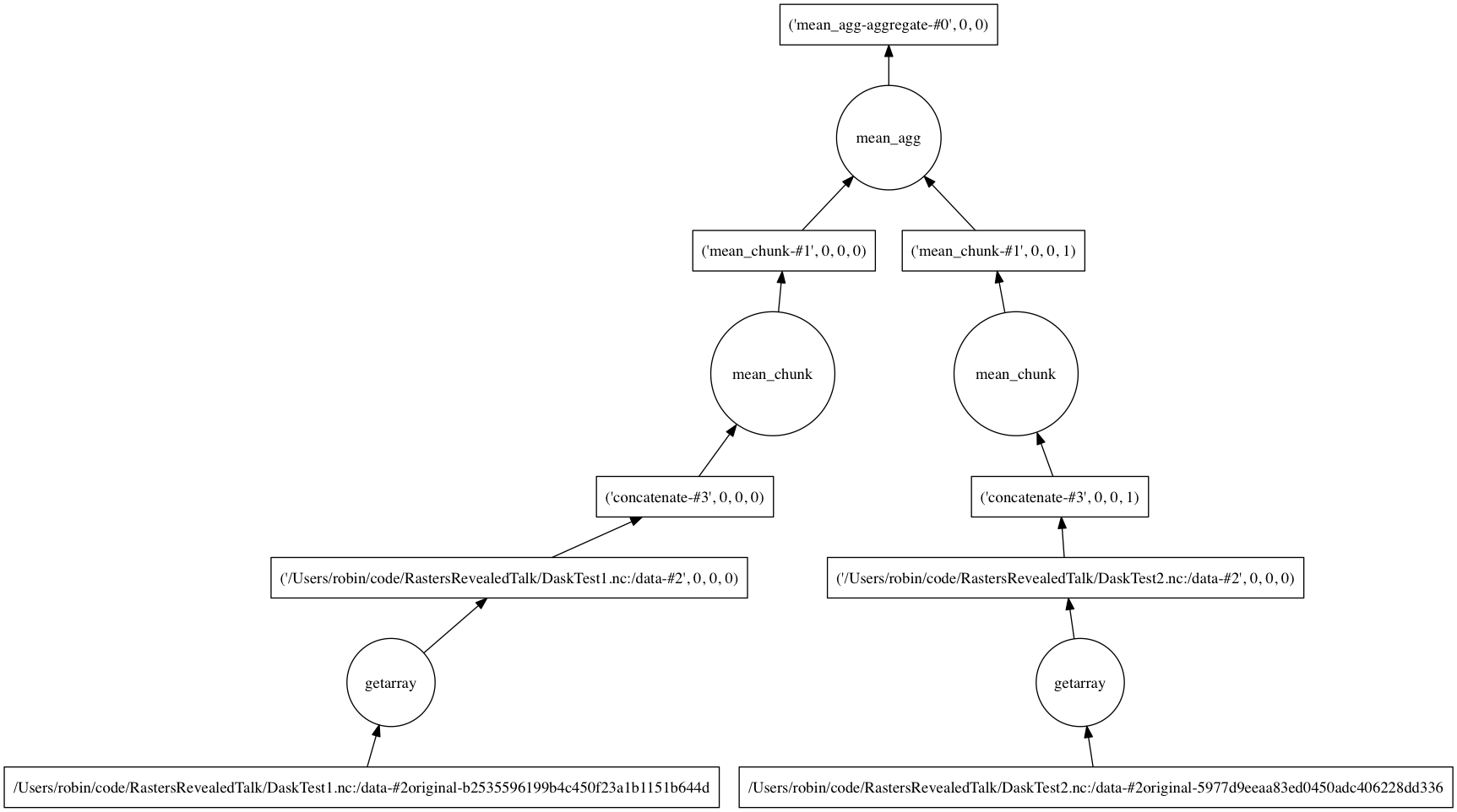
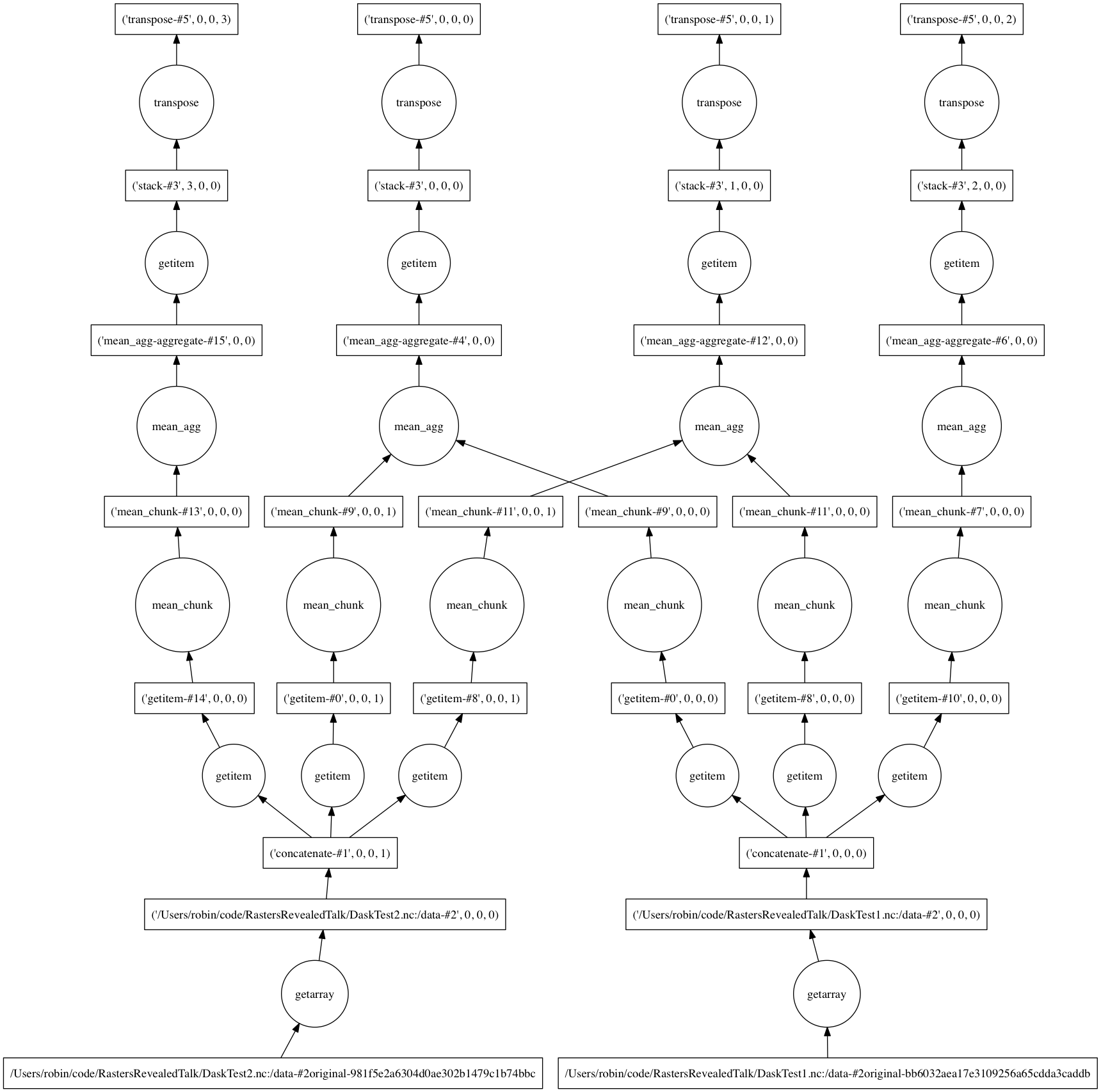
dask creates a computational graph of your processing steps, and then executes it as efficiently as possible.

This includes only loading data that is actually needed and only processing things once.

In [26]:
data = xr.open_mfdataset(['DaskTest1.nc', 'DaskTest2.nc'], chunks={'time':10})['data']
avg = data.mean(dim='time')
In [27]:
seasonal = data.groupby('time.season').mean(dim='time')

dask.distributed

All of these different chunks, and separate processing chains can be run on separate computers.

Getting raster data into xarray

xarray can read various raster formats directly:

  • NetCDF
  • HDF
  • GRIB

However, xarray can't currently read other standard raster formats like:

  • GeoTIFF
  • Erdas IMAGINE
  • Arc Grids
  • ENVI format
  • etc...

rasterio

A nice, Pythonic interface to GDAL - making it really easy to read almost any raster file into Python

In [28]:
import rasterio

with rasterio.open('SPOT_ROI.tif') as src:
    data = src.read(1)
    
print(data)
[[51 51 51 ..., 32 32 29]
 [51 51 51 ..., 29 30 27]
 [54 54 52 ..., 30 29 28]
 ..., 
 [33 34 34 ..., 31 35 35]
 [34 34 34 ..., 32 34 34]
 [34 34 34 ..., 31 33 38]]

Joining them up

All we need to do is write some functions to read from rasterio and create a DataArray

But it's a bit more difficult than that...

  • Need to deal with geographic metadata
  • Geographic co-ordinates
  • Dimension names
In [30]:
data = rasterio_to_xarray('SPOT_ROI.tif')
data
rasterio_to_xarray.py:29: FutureWarning: comparison to `None` will result in an elementwise object comparison in the future.
  data = np.where(data == src.nodata, np.nan, data)
Out[30]:
<xarray.DataArray (y: 1644, x: 1435)>
array([[ 51.,  51.,  51., ...,  32.,  32.,  29.],
       [ 51.,  51.,  51., ...,  29.,  30.,  27.],
       [ 54.,  54.,  52., ...,  30.,  29.,  28.],
       ..., 
       [ 33.,  34.,  34., ...,  31.,  35.,  35.],
       [ 34.,  34.,  34., ...,  32.,  34.,  34.],
       [ 34.,  34.,  34., ...,  31.,  33.,  38.]])
Coordinates:
  * y        (y) float64 1.484e+05 1.484e+05 1.484e+05 1.484e+05 1.484e+05 ...
  * x        (x) float64 4.301e+05 4.301e+05 4.302e+05 4.302e+05 4.302e+05 ...
Attributes:
    crs: +ellps=airy +k=0.999601 +lat_0=49 +lon_0=-2 +no_defs +proj=tmerc +towgs84=446.448,-125.157,542.06,0.15,0.247,0.842,-20.489 +units=m +x_0=400000 +y_0=-100000
    affine: (430130.2396, 10.0, 0.0, 148415.8755, 0.0, -10.0)

Example - combining multiple files into a time-series

Take a large number of files, one from each orbit of a satellite, and put them into one large array with a time dimension.

In [34]:
list_of_data_arrays = [file_to_da(filename) for filename in files]
In [35]:
combined = xr.concat(list_of_data_arrays, dim='time')
In [41]:
combined.shape
Out[41]:
(10, 1162, 1240)
In [42]:
combined.coords
Out[42]:
Coordinates:
  * y        (y) float64 1.429e+06 1.428e+06 1.427e+06 1.426e+06 1.424e+06 ...
  * x        (x) float64 -9.476e+05 -9.464e+05 -9.451e+05 -9.439e+05 ...
  * time     (time) datetime64[ns] 2003-04-16T14:40:00 2002-03-19T11:20:00 ...

Getting raster data out of xarray

In [37]:
mean = combined.mean(dim='time', keep_attrs=True)
In [38]:
xarray_to_rasterio(mean, 'Mean.tif')

Geographic processing

Can xarray do standard geographic processing methods?

  • Zonal statistics
  • Reprojecting
  • etc...
  • A DataArray is just a fancy numpy array
  • Many things will work directly, otherwise just use .values to get the numpy array

Zonal statistics

rasterstats is a Python module for doing zonal statistics

We can use the same approach as the Python module, but modified to work with DataArray objects

Zonal statistics

  1. Load shapefile
  2. For each feature in the shapefile:
    • Rasterize the feature into an array
    • Use this array to index the DataArray
    • Do whatever processing you want (mean, median, std etc)

(There are more efficient ways to do this if no polygons overlap)

And more...

  • Apply functions across axes (eg. linear regression over time, separately for each pixel)
  • Rolling windows over any axis
  • Automatic broadcasting and alignment
  • Hierarchical indexes
  • OPeNDAP

Where next...?

  • xarray is under rapid development
  • General approach is stable, some details may change
  • Very responsive developers
  • Raster I/O will be built-in to xarray soon-ish
  • dask is rapidly improving too

Resources